TL;DR – This is the first article I am writing to report on my journey studying the MPL-Mixer architecture. It will cover the basics up to an intermediate level. The goal is not to reach an advanced level.

Reference: https://arxiv.org/abs/2105.01601

Introduction

From the original paper it’s stated that

We propose the MLP-Mixer architecture (or “Mixer” for short), a competitive but conceptually and technically simple alternative, that does not use convolutions or self-attention. Instead, Mixer’s architecture is based entirely on multi-layer perceptrons (MLPs) that are repeatedly applied across either spatial locations or feature channels. Mixer relies only on basic matrix multiplication routines, changes to data layout (reshapes and transpositions), and scalar nonlinearities.

At first, this explanation wasn’t very intuitive to me. With that in mind, I decided to investigate other resources that could provide an easier explanation. In any case, let’s keep in mind that the proposed architecture is shown in the image below.

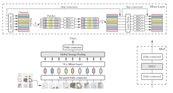
Unlike CNNs, which focus on local image regions through convolutions, and transformers, which use attention to capture relationships between image patches, the MLP-Mixer uses only two types of operations:

• Patch Mixing (Spatial Mixing)
• Channel Mixing

Image Patches

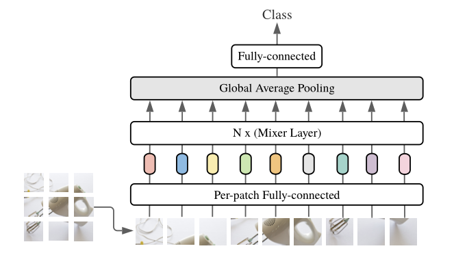
In general, from the figure below, we can see that this architecture is a “fancy” classification model, where the output of the fully connected layer is a class. The input for this architecture is an image, which is divided into patches.

In case you’re not 100% sure what a patch is, when an image is divided into ‘patches,’ it means the image is split into smaller, equally sized square (or rectangular) sections, known as patches. Each patch represents a small, localized region of the original image. Instead of processing the entire image as a whole, these smaller patches are analyzed independently or in groups, often for tasks like object detection, classification, or feature extraction. Each patch is then provided to a “Per-patch Fully-connected” layer and subsequently a “ (Mixer Layer).”

How the MLP-Mixer Processes Patches

For a clear example, let’s take a 224×224 pixel image which can be divided into 16×16 pixel patches, when diving the image we’ll have

   

So, the 224×224 pixel image will be divided into a grid of 14 patches along the width and 14 patched along the height. This results in a 14×14 grid of patches. The total number of patches is then calculated by patches. After diving the image into patches, each patch will contain pixels. These pixel values can be flattened into a 1D vector of length 256.

It’s crucial to note that if the image has multiple channels (like RGB with 3 channels), each patch will actually have values because each pixel in a RGB image has three color channels.

Thus, for an RGB image:

• Each patch can be represented as a vector of 768 values
• We then have 196 patches, each represented by a 768-dimensional vector

Each patch (a 768-dimensional vector in our example) is projected into a higher-dimensional space using a linear layer (MLP). This essentially gives each patch an embedding that is used as the input to the MLP-Mixer. More specifically, after dividing the image into patches, each patch is processed by the Per-patch Fully-connected layer (depicted in the second row).

Per-patch Fully Connected Layer

Each patch is essentially treated as a vector of values, as we have explained before, a 768-dimensional vector in our example. These values are passed through a fully connected linear layer, which transforms them into another vector. This is done for each patch independently. The role of this fully connected layer is to map each patch to a higher-dimensional embedding space, similar to how token embeddings are used in transformers.

N x Mixer Layers

This part shows a set of stacked mixer layers that alternate between two different types of MLP-based operations:

1. Patch Mixing
   • In this layer, the model mixes information between patches. This means it looks at the relationships between patches in the image (i.e., across different spatial locations). It’s achieved through an MLP that treats each patch as a separate entity and computes the interactions between them.
2. Channel Mixing
   • After patch mixing, the channel mixing layer processes the internal information of each patch independently. It looks at the relationships between different pixel values (or channels) within each patch by applying another MLP.

These mixer layers alternate between patch mixing and channel mixing. They are applied N times, where N is a hyperparameter to configure the number of times the layers are repeated. The goal of these layers is to mix both spatial (patch-wise) and channel-wise information across the entire image.

Global Average Pooling

After passing through several mixer layers, a global average pooling layer is applied. This layer helps reduce the dimensionality of the output by averaging the activations across all patches. The global average pooling layer computes the average value across all patches, essentially summarizing the information from all patches into a single vector. This reduces the overall dimensionality and prepares the data for the final classification step. Additionally, it helps aggregate the learned features from the entire image in a more compact way.

Fully Connected Layer for Classification

This layer is responsible for taking the output of the global average pooling and mapping it to a classification label. The fully connected layer takes the averaged features from the global pooling layer and uses them to make a prediction about the class of the image. The number of output units in this layer corresponds to the number of classes in the classification task.

Quick Recap Until Now

1. Input Image: the image is divided into small patches
2. Per-patch Fully Connected Layer: Each patch is processed independently by a fully connected layer to create patch embeddings
3. Mixer Layers: The patches are then passed through a series of mixer layers, where information is mixed spatially (between patches) and channel-wise (within patches)
4. Global Average Pooling: The features from all patches are averaged to summarize the information
5. Fully Connected Layer: Finally, the averaged features are used to predict the class label of the image

Overview of the Mixer Layer Architecture

As stated before, the Mixer Layer architecture consists of two alternating operations:

1. Patch Mixing
2. Channel Mixing

Each mixing state is handled by a MLP, and there are also skip-connections and layer normalization steps included. Let’s go step by step through how an image is processed using as a reference the image shown below:

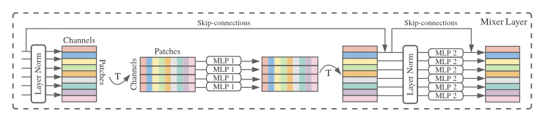
Note, that the image itself is not provided as an input to this diagram. Actually, the image has already been divided into patches as explained before and each patch is processed by a per-patch fully connected layer (linear embedding). The output of that state is what enters the Mixer Layer. Here is how it goes:

• Before reaching this layer, the image has already been divided into patches. These patches are flattened and embedded as vectors (after the per-patch fully connected layer)
• The input to this diagram consists of tokens (one for each patch) and channels (the feature dimensions for each patch)
• So the input is structured as a 2D tensor with:
  • Patches (one patch per token in the sequence)
  • Channels (features within each patch)
• In simple terms, as shown in the image we can think of the input as a matrix where:
  • Each row represents a patch, and
  • Each column represents a channel (feature dimension)

Processing Inside the Mixer Layer

Now, let’s break down the key operations in this Mixer Layer, which processes the patches that come from the previous stage:

1. Layer Normalization
   • The first step is the normalization of the input data to improve training stability. This happens before any mixing occurs.
2. Patch Mixing (First MLP Block)
   • After normalization, the first MLP block is applied. In this operations, the patches are mixed together. The idea here is to capture the relationships between different patches.
   • This operation transposes the input so that it focuses on the patches dimension
   • Then, a MLP is applied along this patches dimension. This is done to allow the model to exchange information between patches and learn how patches relate spatially.
   • Once this mixing is done, the input is transposed back to its original format, where channels are in the focus again.
3. Skip Connection
   • The architecture uses a skip-connection (bypass residual layers, allowing any layer to flow directly to any subsequent layer) that adds the original input (before patch mixing) back to the output of the patch mixing block. This helps avoid degradation of information during training.
4. Layer Normalization
   • Another layer normalization step is applied to the output of the token mixing operation before the next operation (channel mixing) is applied
5. Channel Mixing (Second MLP Block)
   • The second MLP block performs channel mixing. Here, each patch is processed independently by a separate MLP. The goal is to model relationships between the different channels (features) within each patch.
   • The input is processed along the channels dimension (without mixing information between different patches). The MLP learns to capture dependencies between the various features within each patch
6. Skip Connection (for Channel Mixing)
   • Similar to patch mixing, there’s a skip-connection in the channel mixing block as well. This allows the model to retain the original input after the channel mixing operation and helps in stabilizing the learning process.

With the step by step explanation above we can summarize it with some key points:

• Patch Mixing – this part processes the relationships between different patches (spatial mixing), allowing the model to understand global spatial patterns across the image
• Channel Mixing – this part processes the relationships within each patch (channel-wise mixing), learning to capture dependencies between the features (such as pixel intensities or features maps) within each patch
• Skip Connections – The skip connections help the network retain the original input and prevent vanishing gradient problems, especially in deep networks

Inside the MLP Block

The MLP block used in the MLP-Mixer architecture can be seen in the image below:

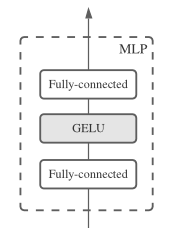
1. Fully Connected Layer
   • The input (whether it’s patch embeddings or channels, depending on the context) first passes through a fully connected layer. This layer performs a linear transformation of the input, meaning it multiplies the input by a weight matrix and adds a bias term.
2. GELU (Gaussian Error Linear Unit) Activation
   • After the first fully connected layer, a GELU activation function is applied. GELU is a non-linear activation function that is smoother than the ReLU. It allows for a more fine-grained activation, as it approximates the behavior of a normal distribution. The formula for GELU is given by

   

where is the cumulative distribution function of a standard Gaussian distribution. The choice of GELU in MLP-Mixer is intended to improve the model’s ability to handle non-linearities in the data, which helps the model learn more complex patterns.

How it works in context:

• In the Token Mixing MLP, this block is applied across the patch (token) dimension, mixing information across different patches
• In the Channel Mixing MLP, the same structure is applied across the channels dimension, mixing the information within each patch independently.

Intuition – The MLP block acts as the core computational unit within the MLP-Mixer. By using two fully connected layers with an activation function in between, it learns to capture both linear and non-linear relationships within the data, depending on where it is applied (either for mixing patches or channels).

Conclusion

The MLP-Mixer offers a unique approach to image classification by leveraging simple multilayer perceptrons (MLPs) for both spatial and channel-wise interactions. By dividing an image into patches and alternating between patch mixing and channel mixing layers, the MLP-Mixer efficiently captures global spatial dependencies and local pixel relationships without relying on traditional convolutional operations. This architecture provides a streamlined yet powerful method for extracting meaningful patterns from images, demonstrating that, even with minimal reliance on complex operations, impressive performance can be achieved in deep learning tasks. It is important to note, however, that this architecture can be applied to different fields, such as time series predictions, even though it was initially proposed for vision tasks.

---

---

If you’ve made it this far, I want to express my gratitude. I hope this has been helpful to someone other than just me!

✧⁺⸜(^-^)⸝⁺✧